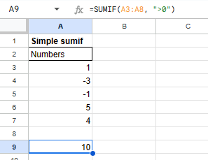
In Google sheets you can use sumif to conditionally sum values in a range depending on a criteria. For example the following formula will sum numbers larger than zero in range A3:A8:
=SUMIF(A3:A8, ">0")
It can be seen on this sheet or in the image below:

As you can see all numbers above zero have been added together, this excludes -1 and -3. For the criteria you can use all the usual comparison operators like =, >, <, >= and <=.
Sum based on criteria from another column
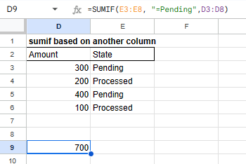
You can also sum based on another column than the one you want to summarise. You can do this by adding one extra parameter to the sumif function to provide which column to use the criterion on. Below is an example:
=SUMIF(E3:E8, "=Pending",D3:D8)
It can be seen on this sheet or in the image below:

In the above we only sum the rows that are pending in the D3:D8 column.
Sum based on criteria matching two or more columns
Sometimes you might want to sum conditionally on multiple other columns, in this scenario you can use sumifs. Below is an example where we only want to sum transactions that are both processed (I3:I8) and paid (J3:J8):
=SUMIFS(H3:H8, I3:I8, "=Processed",J3:J8, "=Paid")
It can be seen on this sheet or in the image below:

In the above there has to be a match on two columns for the numbers to be summed up.
Sum multiple criterias in the same column
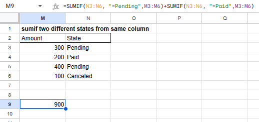
Sometimes you want to sum more than one criteria in a column. I have not been able to find an easy way to do this other than making individual sumifs and adding them together. In the below we sum both Pending (M3:M6) and Paid (M3:M6) transactions together:
=SUMIF(N3:N6, "=Pending",M3:M6)+SUMIF(N3:N6, "=Paid",M3:M6)
It can be seen on this sheet or in the image below:

There are many other ways to do this online using regex and such, but the above is simple and easy to read!
That is all
I hope you enjoyed this post on sumif, you can also check out my post on countif if you only want to count the rows. Feel free to leave a comment down below I read all of them!