Google sheets - How to use vlookup to look up values using a key

In Google sheets you can use VLOOKUP to look up a value based on a key. In short VLOOKUP will search for a specific key in one column and find the value in an adjacent column based on an index. VLOOKUP can be used for several things:

• Data validation, ensuring that entered values match existing data.
• Merge data from multiple sheets or tables by matching a common identifier.
• Or just a simple look up of a value!

The syntax for the VLOOKUP looks like the following VLOOKUP(search_key, range, index, is_sorted):

• search_key: The key you want to search for in the range in the next parameter (range).
• range: The range of cells that will be used for the vlookup. The first column is the one being matched against using the search_key and the value is found in an adjacent column using the index parameter.
• index: The index is the column number (starting from 1) from which you want to retrieve the value. The first column is the same that the search_key is matched on, the next column is the 2nd column in the range and so forth.
• is_sorted: An optional parameter that indicates whether the data range is sorted in ascending order. Set this to TRUE for sorted data or FALSE for unsorted data. If the data is not sorted and you set is_sorted to TRUE you might fail to retrieve values and get an error.

All examples in this post can be found here.

We will use a simple example of cars and look up their prices. A simple example of VLOOKUP could be written as =VLOOKUP(E2,A2:B4, 2, false):

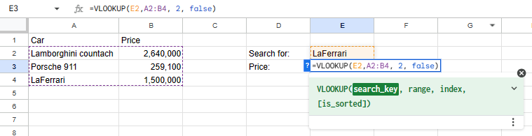
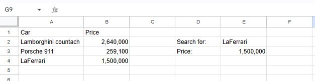
In the above example, E2 is the search_key, A2:B2 is a range containing the column to match on and value column, 2 is the index of the value column and is_sorted is set to false. The result of this query will be 1.500.000:

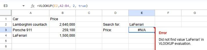
If we set the =VLOOKUP(E2,A2:B4, 2, true) the above function will fail with N/A:

It is a good practice to handle these sorts of errors and this can be done using IFERROR, an example could be =IFERROR(VLOOKUP(E2,A2:B4, 2, true), "Value not found"):

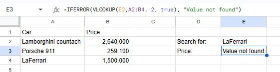
The above return an error message if the value is not found, if the value is found it is returned instead.

That is all

All examples in this post can be found here.

I hope you enjoyed this post on the use of VLOOKUP, please leave a comment down below with your thoughts or if this was helpful!